Deep Dive into MySQL 5.5 Partitioning Enhancements

MySQL 5.5 Partitioning Enhancements: A Guide to Non-Integer Columns, Multi-Column Partitioning, and More

The release of MySQL 5.5 brought many enhancements. While much has been reported on features like semi-synchronous replication, the partitioning enhancements have often been overlooked, and sometimes their true significance has been misunderstood. In this article, we hope to explain these cool enhancements, especially the parts most of us haven’t fully grasped yet. 51CTO recommends the MySQL Database Introduction and Mastery Tutorial.
Figure 1 You haven’t noticed yet that my MySQL partitioning feature is also very strong, eh
Non-Integer Column Partitioning
Anyone who has used partitioning has likely encountered numerous issues, particularly when dealing with non-integer column partitioning. MySQL 5.1 could only handle partitioning on integer columns. If you wanted to partition on a date or string column, you had to use functions to convert them.
MySQL 5.5 introduces two new partitioning methods, RANGE and LIST partitioning, along with a new COLUMNS keyword in the function. Let’s assume we have a table like this:

1. CREATE TABLE expenses (
2. expense_date DATE NOT NULL,
3. category VARCHAR(30),
4. amount DECIMAL (10,3)
5. );

If you wanted to use the partition types available in MySQL 5.1, you would have to convert the types to integers, potentially requiring an additional lookup table. With MySQL 5.5, you can forego the type conversion, like so:

1. ALTER TABLE expenses
2. PARTITION BY LIST COLUMNS (category)
3. (
4. PARTITION p01 VALUES IN ( ‘lodging’, ‘food’),
5. PARTITION p02 VALUES IN ( ‘flights’, ‘ground transportation’),
6. PARTITION p03 VALUES IN ( ‘leisure’, ‘customer entertainment’),
7. PARTITION p04 VALUES IN ( ‘communications’),
8. PARTITION p05 VALUES IN ( ‘fees’)
9. );

Such a partitioning statement is not only more readable but also makes data organization and management very clear. The example above only partitions on the category column.
Another headache when using partitioning in MySQL 5.1 was the date type (i.e., date columns). You couldn’t use them directly; you had to convert these columns using YEAR or TO_DAYS, like this:

1. /* In MySQL 5.1 */
2. CREATE TABLE t2
3. (
4. dt DATE
5. )
6. PARTITION BY RANGE (TO_DAYS(dt))
7. (
8. PARTITION p01 VALUES LESS THAN (TO_DAYS(‘2007-01-01’)),
9. PARTITION p02 VALUES LESS THAN (TO_DAYS(‘2008-01-01’)),
10. PARTITION p03 VALUES LESS THAN (TO_DAYS(‘2009-01-01’)),
11. PARTITION p04 VALUES LESS THAN (MAXVALUE));
13. SHOW CREATE TABLE t2 /G
14. *************************** 1. row ***************************
15. Table: t2
16. Create Table: CREATE TABLE `t2` (
17. `dt` date DEFAULT NULL
18. ) ENGINE=MyISAM DEFAULT CHARSET=latin1
19. /*!50100 PARTITION BY RANGE (TO_DAYS(dt))
20. (PARTITION p01 VALUES LESS THAN (733042) ENGINE = MyISAM,
21. PARTITION p02 VALUES LESS THAN (733407) ENGINE = MyISAM,
22. PARTITION p03 VALUES LESS THAN (733773) ENGINE = MyISAM,
23. PARTITION p04 VALUES LESS THAN MAXVALUE ENGINE = MyISAM) */

This looks terrible. Of course, there are workarounds, but they introduce a lot of trouble. Defining a partition using YEAR or TO_DAYS is indeed confusing, and you had to use the bare column in queries because queries with functions cannot recognize partitions.
But the situation has changed dramatically in MySQL 5.5. You can now partition directly on date columns, and the method is straightforward.

1. /* In MySQL 5.5 */
2. CREATE TABLE t2
3. (
4. dt DATE
5. )
6. PARTITION BY RANGE COLUMNS (dt)
7. (
8. PARTITION p01 VALUES LESS THAN (‘2007-01-01’),
9. PARTITION p02 VALUES LESS THAN (‘2008-01-01’),
10. PARTITION p03 VALUES LESS THAN (‘2009-01-01’),
11. PARTITION p04 VALUES LESS THAN (MAXVALUE));
13. SHOW CREATE TABLE t2 /G
14. *************************** 1. row ***************************
15. Table: t2
16. Create Table: CREATE TABLE `t2` (
17. `dt` date DEFAULT NULL
18. ) ENGINE=MyISAM DEFAULT CHARSET=latin1
19. /*!50500 PARTITION BY RANGE COLUMNS(dt)
20. (PARTITION p01 VALUES LESS THAN (‘2007-01-01’) ENGINE = MyISAM,
21. PARTITION p02 VALUES LESS THAN (‘2008-01-01’) ENGINE = MyISAM,
22. PARTITION p03 VALUES LESS THAN (‘2009-01-01’) ENGINE = MyISAM,
23. PARTITION p04 VALUES LESS THAN (MAXVALUE) ENGINE = MyISAM) */

Here, there is no conflict between definition by function and query by column, because it is defined by column, and the values we insert in the definition are preserved.
Multi-Column Partitioning
The COLUMNS keyword now allows string and date columns as partition definition columns, and it also allows you to use multiple columns to define a partition. You may have seen some examples in the official documentation, such as:

1. CREATE TABLE p1 (
2. a INT,
3. b INT,
4. c INT
5. )
6. PARTITION BY RANGE COLUMNS (a,b)
7. (
8. PARTITION p01 VALUES LESS THAN (10,20),
9. PARTITION p02 VALUES LESS THAN (20,30),
10. PARTITION p03 VALUES LESS THAN (30,40),
11. PARTITION p04 VALUES LESS THAN (40,MAXVALUE),
12. PARTITION p05 VALUES LESS THAN (MAXVALUE,MAXVALUE)
13. );
15. CREATE TABLE p2 (
16. a INT,
17. b INT,
18. c INT
19. )
20. PARTITION BY RANGE COLUMNS (a,b)
21. (
22. PARTITION p01 VALUES LESS THAN (10,10),
23. PARTITION p02 VALUES LESS THAN (10,20),
24. PARTITION p03 VALUES LESS THAN (10,30),
25. PARTITION p04 VALUES LESS THAN (10,MAXVALUE),
26. PARTITION p05 VALUES LESS THAN (MAXVALUE,MAXVALUE)
27. )

Similarly, there are other examples like PARTITION BY RANGE COLUMNS (a,b,c). Because I used MySQL 5.1 partitioning for a long time, I didn’t quite grasp the meaning of multi-column partitioning. What does LESS THAN (10,10) mean? What happens if the next partition is LESS THAN (10,20)? Conversely, what about (20,30)?
All these questions need an answer, and before answering, we need to better understand what we are doing.
It might be confusing at first. When all partitions have a different range of values, it might seem like it’s actually partitioning on just one column of the table. But this is not the case. Consider the following example:

1. CREATE TABLE p1_single (
2. a INT,
3. b INT,
4. c INT
5. )
6. PARTITION BY RANGE COLUMNS (a)
7. (
8. PARTITION p01 VALUES LESS THAN (10),
9. PARTITION p02 VALUES LESS THAN (20),
10. PARTITION p03 VALUES LESS THAN (30),
11. PARTITION p04 VALUES LESS THAN (40),
12. PARTITION p05 VALUES LESS THAN (MAXVALUE)
13. );

This is different from the previous table p1. If you insert (10,1,1) into table p1, it will go into the first partition. Conversely, in table p1_single, it will go into the second partition. The reason is that (10,1) is less than (10,10). If you only focus on the first value, you haven’t realized that you are comparing a tuple, not a single value.
Now let’s analyze the trickiest part. What happens when you need to determine where a certain row should go? How do you evaluate an operation like (10,9) < (10,10)? The answer is actually quite simple. You evaluate the two records the same way you would when sorting them.

1. a=10
2. b=9
3. (a,b) < (10,10) ?
5. # evaluates to:
7. (a < 10)
8. OR
9. ((a = 10) AND ( b < 10))
11. # which translates to:
13. (10 < 10)
14. OR
15. ((10 = 10) AND ( 9 < 10))

If there are three columns, the expression gets longer, but not more complex. You first test for less-than on the first item. If two or more partitions match, then you test the second item. If more than one candidate partition remains, you then test the third item.
The figure shown below illustrates the traversal of three records being inserted into partitions defined with the following code:
(10,10),
(10,20),
(10,30),
(10, MAXVALUE)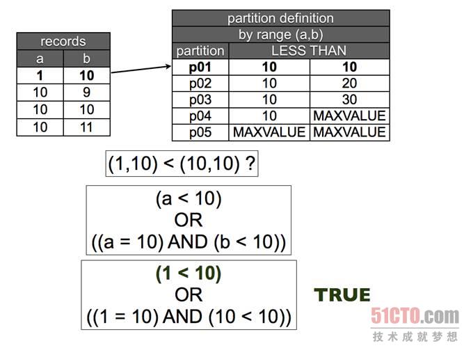

Figure 2 Tuple comparison. When the first value is less than the first range defined by the partition, then the row belongs here.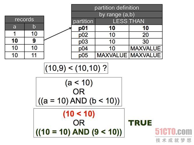

Figure 3 Tuple comparison. When the first value equals the first range defined by the partition, we need to compare the second item. If it’s less than the second range, then the row belongs here.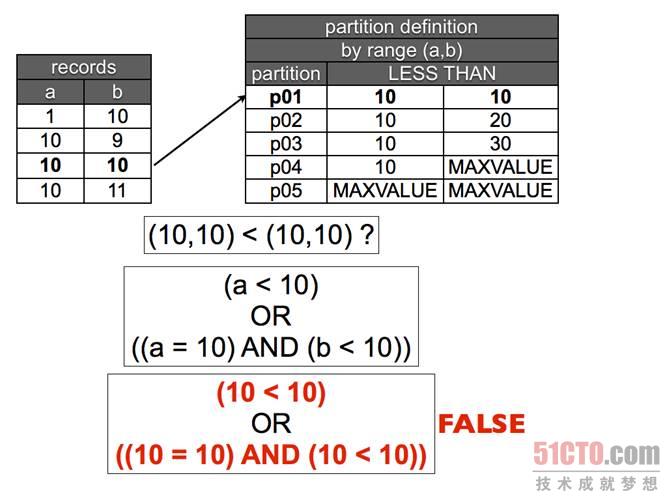

Figure 4 Tuple comparison. When the first value and the second value equal their corresponding ranges, if the tuple is not less than the defined range, then it does not belong here; continue to the next step.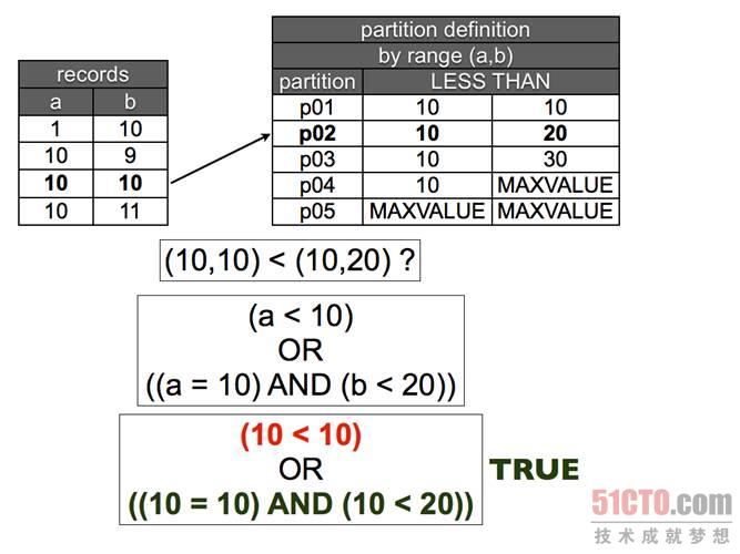

Figure 5 Tuple comparison. At the next range, the first item is equal, and the second item is less than, therefore the tuple is smaller, and the row belongs here.
With the help of these diagrams, we have a deeper understanding of the steps involved in inserting a record into a multi-column partitioned table. This is all theoretical. To help you better grasp the new feature, let’s look at a slightly more advanced example, one that is more meaningful for the pragmatic reader. Here is the table definition script:

1. CREATE TABLE employees (
2. emp_no int(11) NOT NULL,
3. birth_date date NOT NULL,
4. first_name varchar(14) NOT NULL,
5. last_name varchar(16) NOT NULL,
6. gender char(1) DEFAULT NULL,
7. hire_date date NOT NULL
8. ) ENGINE=MyISAM
9. PARTITION BY RANGE COLUMNS(gender,hire_date)
10. (PARTITION p01 VALUES LESS THAN (‘F’,’1990-01-01′) ,
11. PARTITION p02 VALUES LESS THAN (‘F’,’2000-01-01′) ,
12. PARTITION p03 VALUES LESS THAN (‘F’,MAXVALUE) ,
13. PARTITION p04 VALUES LESS THAN (‘M’,’1990-01-01′) ,
14. PARTITION p05 VALUES LESS THAN (‘M’,’2000-01-01′) ,
15. PARTITION p06 VALUES LESS THAN (‘M’,MAXVALUE) ,
16. PARTITION p07 VALUES LESS THAN (MAXVALUE,MAXVALUE)

Unlike the examples above, this one is easier to understand. The first partition stores female employees hired before 1990. The second partition stores female employees hired between 1990 and 2000. The third partition stores all remaining female employees. For partitions p04 to p06, the strategy is the same, but for male employees. The last partition is a catch-all.
After reading this, you might ask, how do I know which partition a row is stored in? There are two methods. The first is to query using the same conditions as the partition definition as the query condition.

1. SELECT
2. CASE
3. WHEN gender = ‘F’ AND hire_date < '1990-01-01'
4. THEN ‘p1’
5. WHEN gender = ‘F’ AND hire_date < '2000-01-01'
6. THEN ‘p2’
7. WHEN gender = ‘F’ AND hire_date < '2999-01-01'
8. THEN ‘p3’
9. WHEN gender = ‘M’ AND hire_date < '1990-01-01'
10. THEN ‘p4’
11. WHEN gender = ‘M’ AND hire_date < '2000-01-01'
12. THEN ‘p5’
13. WHEN gender = ‘M’ AND hire_date < '2999-01-01'
14. THEN ‘p6’
15. ELSE
16. ‘p7’
17. END as p,
18. COUNT(*) AS rows
19. FROM employees
20. GROUP BY p;
22. +——+——-+
23. | p | rows |
24. +——+——-+
25. | p1 | 66212 |
26. | p2 | 53832 |
27. | p3 | 7 |
28. | p4 | 98585 |
29. | p5 | 81382 |
30. | p6 | 6 |
31. +——+——-+

If the table is MyISAM or ARCHIVE, you can trust the statistical information provided by INFORMATION_SCHEMA.

1. SELECT
2. partition_name part,
3. partition_expression expr,
4. partition_description descr,
5. table_rows
6. FROM
7. INFORMATION_SCHEMA.partitions
8. WHERE
9. TABLE_SCHEMA = schema()
10. AND TABLE_NAME=’employees’;
11. +——+——————+——————-+————+
12. | part | expr | descr | table_rows |
13. +——+——————+——————-+————+
14. | p01 | gender,hire_date | ‘F’,’1990-01-01′ | 66212 |
15. | p02 | gender,hire_date | ‘F’,’2000-01-01′ | 53832 |
16. | p03 | gender,hire_date | ‘F’,MAXVALUE | 7 |
17. | p04 | gender,hire_date | ‘M’,’1990-01-01′ | 98585 |
18. | p05 | gender,hire_date | ‘M’,’2000-01-01′ | 81382 |
19. | p06 | gender,hire_date | ‘M’,MAXVALUE | 6 |
20. | p07 | gender,hire_date | MAXVALUE,MAXVALUE | 0 |
21. +——+——————+——————-+————+

If the storage engine is InnoDB, the values above are approximate. If you need exact values, you cannot trust them.
Another question is about its performance. Do these enhancements trigger partition pruning? The answer is unequivocally yes. Unlike MySQL 5.1, where date partitioning only worked with two functions, in MySQL 5.5, any partition defined using the COLUMNS keyword can utilize partition pruning. Let’s test it out below.

1. select count(*) from employees where gender=’F’ and hire_date < '1990-01-01';
2. +———-+
3. | count(*) |
4. +———-+
5. | 66212 |
6. +———-+
7. 1 row in set (0.05 sec)
9. explain partitions select count(*) from employees where gender=’F’ and hire_date < '1990-01-01'/G
10. *************************** 1. row ***************************
11. id: 1
12. select_type: SIMPLE
13. table: employees
14. partitions: p01
15. type: ALL
16. possible_keys: NULL
17. key: NULL
18. key_len: NULL
19. ref: NULL
20. rows: 300024
21. Extra: Using where

By using the conditions that define the first partition, we achieved a highly optimized query. More than that, partial conditions will also benefit from partition pruning.

1. select count(*) from employees where gender=’F’;
2. +———-+
3. | count(*) |
4. +———-+
5. | 120051 |
6. +———-+
7. 1 row in set (0.12 sec)
9. explain partitions select count(*) from employees where gender=’F’/G
10. *************************** 1. row ***************************
11. id: 1
12. select_type: SIMPLE
13. table: employees
14. partitions: p01,p02,p03,p04
15. type: ALL
16. possible_keys: NULL
17. key: NULL
18. key_len: NULL
19. ref: NULL
20. rows: 300024
21. Extra: Using where

It follows the same algorithm as a composite index. If your condition refers to the leftmost part of the index, MySQL will use it. Similarly, if your condition refers to the leftmost part of the partition definition, MySQL will prune as much as possible. It works alongside composite indexes, so if you only use the rightmost condition, partition pruning will not work.

1. select count(*) from employees where hire_date < '1990-01-01';
2. +———-+
3. | count(*) |
4. +———-+
5. | 164797 |
6. +———-+
7. 1 row in set (0.18 sec)
9. explain partitions select count(*) from employees where hire_date < '1990-01-01'/G
10. *************************** 1. row ***************************
11. id: 1
12. select_type: SIMPLE
13. table: employees
14. partitions: p01,p02,p03,p04,p05,p06,p07
15. type: ALL
16. possible_keys: NULL
17. key: NULL
18. key_len: NULL
19. ref: NULL
20. rows: 300024
21. Extra: Using where

If you don’t use the first part of the partition definition, and instead use the second part, a full table scan will occur. Always keep this in mind when designing partitions and writing queries.
Usability Enhancement: Truncate Partition
One of the most attractive features of partitioning is the ability to instantly remove a massive number of records. DBAs love to store historical records in tables partitioned by date, allowing them to periodically delete outdated historical data. This method works quite well. Assuming the first partition stores the oldest historical records, you can simply drop the first partition, then create a new partition at the end to hold the most recent historical records. This cycle enables fast purging of historical records.
But when you need to remove only part of the data from a partition, things are not so simple. Dropping a partition is no problem, but emptying a partition is a headache. To remove all data from a partition while keeping the partition itself, you could:
Use a DELETE statement, but we know DELETE statements have notoriously poor performance.
Use a DROP PARTITION statement, followed by a REORGANIZE PARTITIONS statement to recreate the partition, but the cost of doing this is much higher than the previous method.
MySQL 5.5 introduces TRUNCATE PARTITION, which is somewhat similar to the DROP PARTITION statement but retains the partition itself, meaning the partition can be reused. TRUNCATE PARTITION should be a mandatory tool in any DBA’s toolkit.
More Fine-Tuning Features: TO_SECONDS
The partitioning enhancement package includes a new function for handling DATE and DATETIME columns. Using the TO_SECONDS function, you can convert date/time columns into the number of seconds since year 0. If you want to partition using intervals smaller than one day, this function can help you do just that.
TO_SECONDS triggers partition pruning, and unlike TO_DAYS, it can work in reverse, namely FROM_DAYS. There is no such reverse function for TO_SECONDS, but it’s not difficult to DIY one yourself.

1. drop function if exists from_seconds;
3. delimiter //
4. create function from_seconds (secs bigint)
5. returns DATETIME
6. begin
7. declare days INT;
8. declare secs_per_day INT;
9. DECLARE ZH INT;
10. DECLARE ZM INT;
11. DECLARE ZS INT;
12. set secs_per_day = 60 * 60 * 24;
13. set days = floor(secs / secs_per_day);
14. set secs = secs – (secs_per_day * days);
15. set ZH = floor(secs / 3600);
16. set ZM = floor(secs / 60) – ZH * 60;
17. set ZS = secs – (ZH * 3600 + ZM * 60);
18. return CAST(CONCAT(FROM_DAYS(days), ‘ ‘, ZH, ‘:’, ZM, ‘:’, ZS) as DATETIME);
19. end //
21. delimiter ;

With these new weapons, we can confidently create a temporary partition that is smaller than one day, like so:

1. CREATE TABLE t2 (
2. dt datetime
3. )
4. PARTITION BY RANGE (to_seconds(dt))
5. (
6. PARTITION p01 VALUES LESS THAN (to_seconds(‘2009-11-30 08:00:00’)) ,
7. PARTITION p02 VALUES LESS THAN (to_seconds(‘2009-11-30 16:00:00’)) ,
8. PARTITION p03 VALUES LESS THAN (to_seconds(‘2009-12-01 00:00:00’)) ,
9. PARTITION p04 VALUES LESS THAN (to_seconds(‘2009-12-01 08:00:00’)) ,
10. PARTITION p05 VALUES LESS THAN (to_seconds(‘2009-12-01 16:00:00’)) ,
11. PARTITION p06 VALUES LESS THAN (MAXVALUE)
12. );
13. show create table t2/G
14. *************************** 1. row ***************************
15. Table: t2
16. Create Table: CREATE TABLE `t2` (
17. `dt` datetime DEFAULT NULL
18. ) ENGINE=MyISAM DEFAULT CHARSET=latin1
19. /*!50500 PARTITION BY RANGE (to_seconds(dt))
20. (PARTITION p01 VALUES LESS THAN (63426787200) ENGINE = MyISAM,
21. PARTITION p02 VALUES LESS THAN (63426816000) ENGINE = MyISAM,
22. PARTITION p03 VALUES LESS THAN (63426844800) ENGINE = MyISAM,
23.  PARTITION p04 VALUES LESS THAN (63426873600) ENGINE = MyISAM,  
24.  PARTITION p05 VALUES LESS THAN (63426902400) ENGINE = MyISAM,  
25.  PARTITION p06 VALUES LESS THAN MAXVALUE ENGINE = MyISAM) */ 

Since we did not use the COLUMNS keyword — and we could not use it here because it does not support mixing columns and functions — the recorded values in the table definition are simply the computed results of the TO_SECONDS function.
But thanks to the new function, we can reverse this value and convert it into a much more readable date.

1. select 
2.   partition_name part,  
3.   partition_expression expr,  
4.   from_seconds(partition_description) descr,  
5.   table_rows  
6. FROM 
7. INFORMATION_SCHEMA.partitions  
8. WHERE 
9.     TABLE_SCHEMA = 'test' 
10.     AND TABLE_NAME='t2';  
11. +——+—————-+———————+————+  
12. | part | expr           | descr               | table_rows |  
13. +——+—————-+———————+————+  
14. | p01  | to_seconds(dt) | 2009-11-30 08:00:00 |          0 |  
15. | p02  | to_seconds(dt) | 2009-11-30 16:00:00 |          0 |  
16. | p03  | to_seconds(dt) | 2009-12-01 00:00:00 |          0 |  
17. | p04  | to_seconds(dt) | 2009-12-01 08:00:00 |          0 |  
18. | p05  | to_seconds(dt) | 2009-12-01 16:00:00 |          0 |  
19. | p06  | to_seconds(dt) | 0000-00-00 00:00:00 |          0 |  
20. +——+—————-+———————+————+ 

Summary
MySQL 5.5 is definitely great news for partitioning users. While it may not offer a direct method for performance enhancement (if you measure performance by response time), the easier-to-use enhancements and the TRUNCATE PARTITION command can save DBAs a tremendous amount of time, and sometimes end users as well.
These enhanced features may see updates in the next milestone release, with the final version expected in mid-2010. All partitioning users should give it a try then!
Original source: http://dev.mysql.com/tech-resources/articles/mysql_55_partitioning.html
Original title: A deep look at MySQL 5.5 partitioning enhancements
Author: Giuseppe